

João de Deus

Bruno Teixeira
Our AI-generated summary
Our AI-generated summary
Why Scheduling Is Harder Than It Looks
Production scheduling is one of the most common optimization problems in the industrial landscape. Done well, it can produce tangible business improvements, such as better service levels, or increased machine efficiency by reducing setup times. However, solving these problems is not as easy as you may think.
In the paper industry, specifically, the problem of scheduling the converting lines, where we cut the big rolls of paper into the paper sheets we use every day, is extremely complex, with multiple machines, multiple SKUs, and multiple interdependent decisions. The problem becomes increasingly challenging as we are often met with maximum run times for our algorithms to solve, due to practical industrial limitations.
The real example we bring here involves sequencing over 100 jobs on 6 machines over one week, in one of the world’s largest paper manufacturers. The schedules are also subject to a set of common production and planning constraints, such as stock dependency from previous machines, machines’ availability, sequence-dependent setups between orders… you get the point. All of this while trying to balance stock levels, service levels, and machine efficiency!
The Limits of Classic Optimization
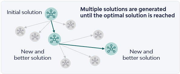
Classic optimization, in this context, means mathematically formulating the problem as a MILP (Mixed-Integer Linear Programming) and feeding it to a solver that iteratively improves the solution and, given enough time, can find the absolute optimal solution. A simple explanation of how these models work is in the image below. As you can imagine, for an optimization solver to iteratively improve a solution it must first find one, and that can be difficult for large, complex problems. For instance, for a scheduling optimization problem the number of decision variables — what defines our solution space — explodes with an increasing number of jobs. Our problem had around 30,000 decision variables for 100 jobs, if this number doubles and we schedule 200 jobs, we would be sitting on around 110,000 decision variables.
Our AI-generated summary
Our AI-generated summary
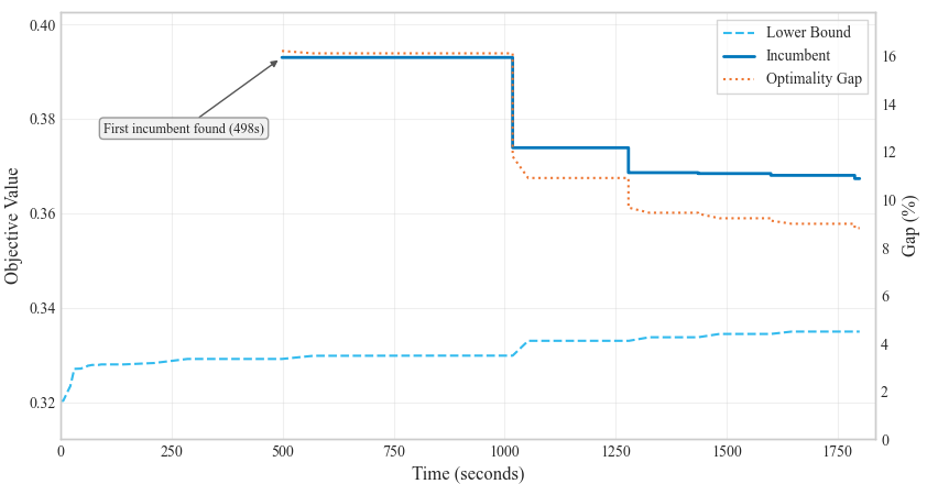
Nonetheless, we first tried to solve the problem at hand using classic exact optimization, with the Gurobi solver, and we stumbled into a wall we could already see from the distance: finding an initial solution for the model to work upon was hard. Almost 30% of the total runtime was spent just trying to find the first solution.
Flipping the Strategy: Global Search Before Local Optimization
At this point we started to think of what other strategies one could possibly use to tackle this situation. We decided to flip the strategy: first search globally and quickly find an initial solution — which we knew would be suboptimal, but feasible — and then optimize locally with a MILP solver to improve optimality.
Finding an initial solution quickly could be achieved through the use of widely studied metaheuristics, which can prove extremely useful in producing powerful solutions in short periods of time, but cannot reach optimality. Therefore, we chose one of the most widely used metaheuristics: a Genetic Algorithm (GA).
Designing an Evolutionary Warm Start
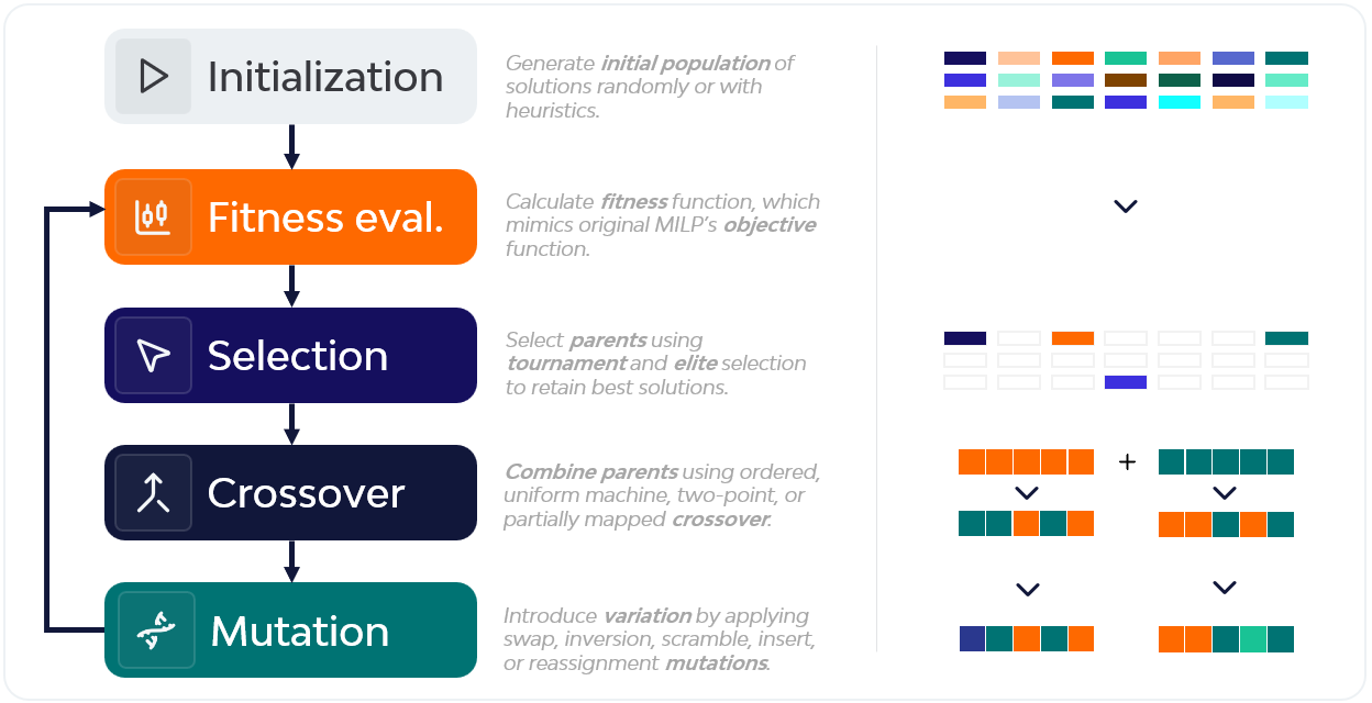
A Genetic Algorithm is an evolutionary algorithm that mimics the dynamics of natural selection. It starts with a population of candidate solutions, called chromosomes, that evolve over generations. For instance, in this case, one chromosome encodes a full weekly sequence of orders across the 6 lines.
In each generation we select the best individuals, recombine them through crossover, and introduce variation through mutation operations. The main goal is to improve the fitness function, which in our case mirrors the MILP’s objective function. A simplified version of the Genetic Algorithm we designed is illustrated below:
On top of the traditional GA, we added a small Q-learning reinforcement component to choose crossover and mutation operators in a smarter way instead of randomly. We also tuned the GA’s parameters using the Taguchi method, which drastically reduced the number of parameter combinations we had to test.
Refining the Solution: Fix-and-Optimize
The GA was able to generate a feasible solution quickly. Though it was nowhere near the optimal solution.
We must now use the created solution to warm start a MILP model, to improve optimality. For this, we opted for two strategies:
- Using the GA warm start solution to feed a classic optimization solver
- Using the GA warm start solution to feed a Fix-and-Optimize heuristic
The Fix-and-Optimize (F&O) heuristic works by iteratively fixing a percentage of the decision variables and letting the solver re-optimize the remaining “free” variables, exploring a local neighborhood around the current best solution.
How the Hybrid Pipeline Works
If you’re curious about how this looks end-to-end, here’s a simplified pseudo-code version of the pipeline:
1: Start timer
2: population ← InitializePopulation(problem data)
3: EvaluateFitness(population)
4: x* ← BestIndividual(population)
5: while elapsed_time < ga_time do
6: parents ← SelectParents(population)
7: offspring ← ApplyCrossoverAndMutation(parents, Q-learning, GA parameters)
8: EvaluateFitness(offspring)
9: population ← FormNewPopulation(population, offspring)
10: x* ← UpdateBest(population, x*)
11: end while
12: remaining_time ← total_time − elapsed_time
13: if solving_mode = EXACT then
14: x* ← SolveFullMILP(problem data, warm_start = x*, time_limit = remaining_time)
15: else
16: for each stage in F&O_stages do
17: for iter = 1 to stage.iterations do
18: FixSubsetOfJobs(stage.fix_percentage, based_on = x*)
19: candidate ← SolveSubMIP(problem data, warm_start = x*, time_limit = stage.time)
20: if Objective(candidate) < Objective(x*) then x* ← candidate
21: end for
22: end for
23: end if
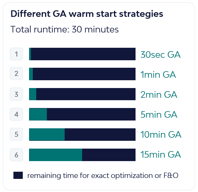
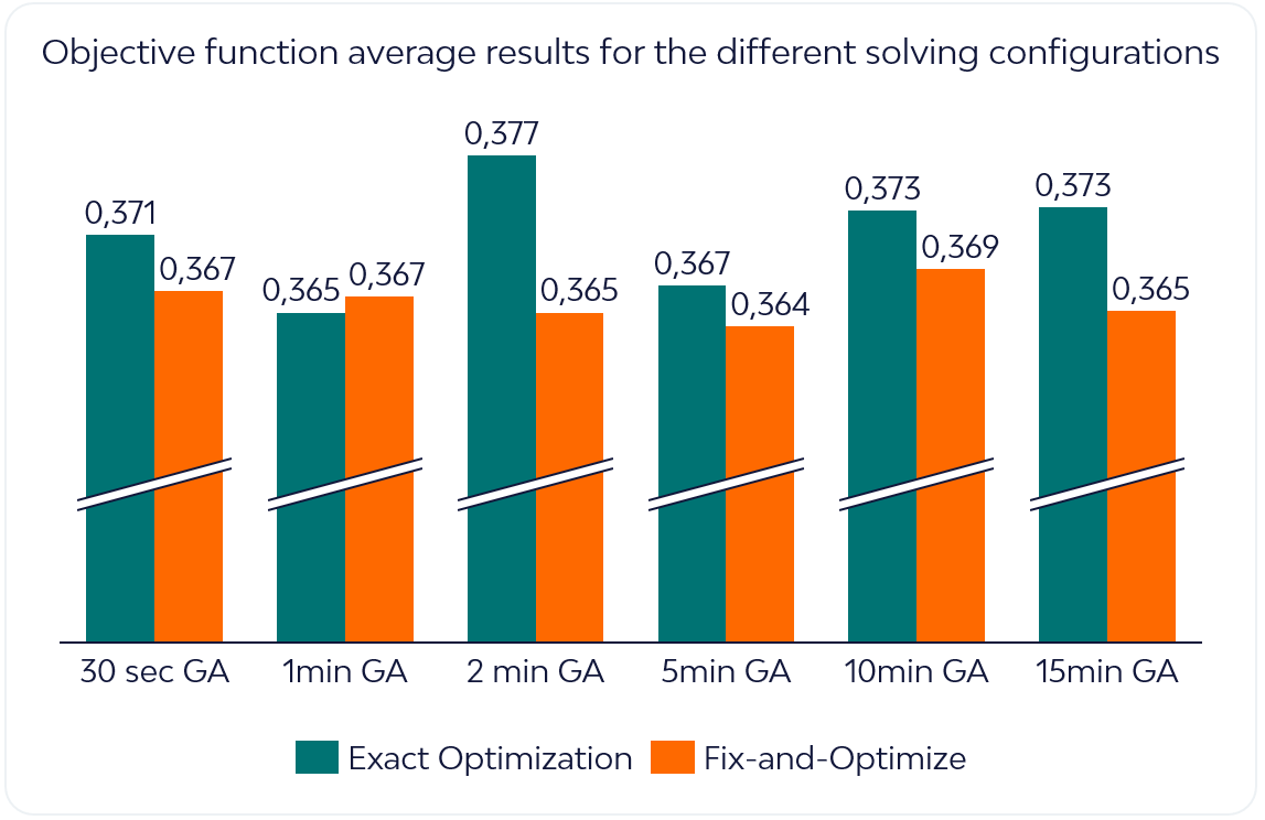
24: return x* Another decision we explored was how much time we should let the Genetic Algorithm run to create the warm start solution, given a strict 30-minute total time limit. Thus, we considered six different approaches by letting the GA run for 30s, 1min, 2min, 5min, 10min, and 15min, with the remaining time used for either Fix-and-Optimize or exact optimization:
A series of tests were performed to assess how each of the two approaches, GA warm start followed by either exact optimization or the Fix-and-Optimize heuristic, behaved for the different warm start duration times. Results are reported on the graphic below. The model in question was a minimization problem, so lower objective values correspond to better solutions.
What Actually Worked (And Why)
Average results show that the Fix-and-Optimize paired with the Genetic Algorithm outperformed the Exact Optimization with GA approach on almost all different warm start approaches. The Fix-and-Optimize approach achieves the best results with the 5-minute GA warm-start.
Intuitively, shorter warm start intervals left the F&O heuristic with too little structural guidance and resulted in worse solutions, while longer intervals warm start the algorithm with better incumbents but leave too little time for MILP refinement. Somewhere in the middle there is a sweet spot.
In conclusion, for complex combinatorial problems, like production scheduling, we can combine the strengths of metaheuristics with MILP solvers to reach better solutions, especially within strict solving time caps. Specifically, for problems where the solution space is so big that solvers get a hard time finding an initial feasible solution, this hybrid approach is definitely worth considering. In our case, metaheuristics didn’t replace the MILP solver, they made it usable at the scale we needed.